PyTorch Quick Tutorial (1)
- 8 minsInstallation
Go to https://pytorch.org/get-started/locally/, select the corresponding options, and install pytorch in the target conda environment:
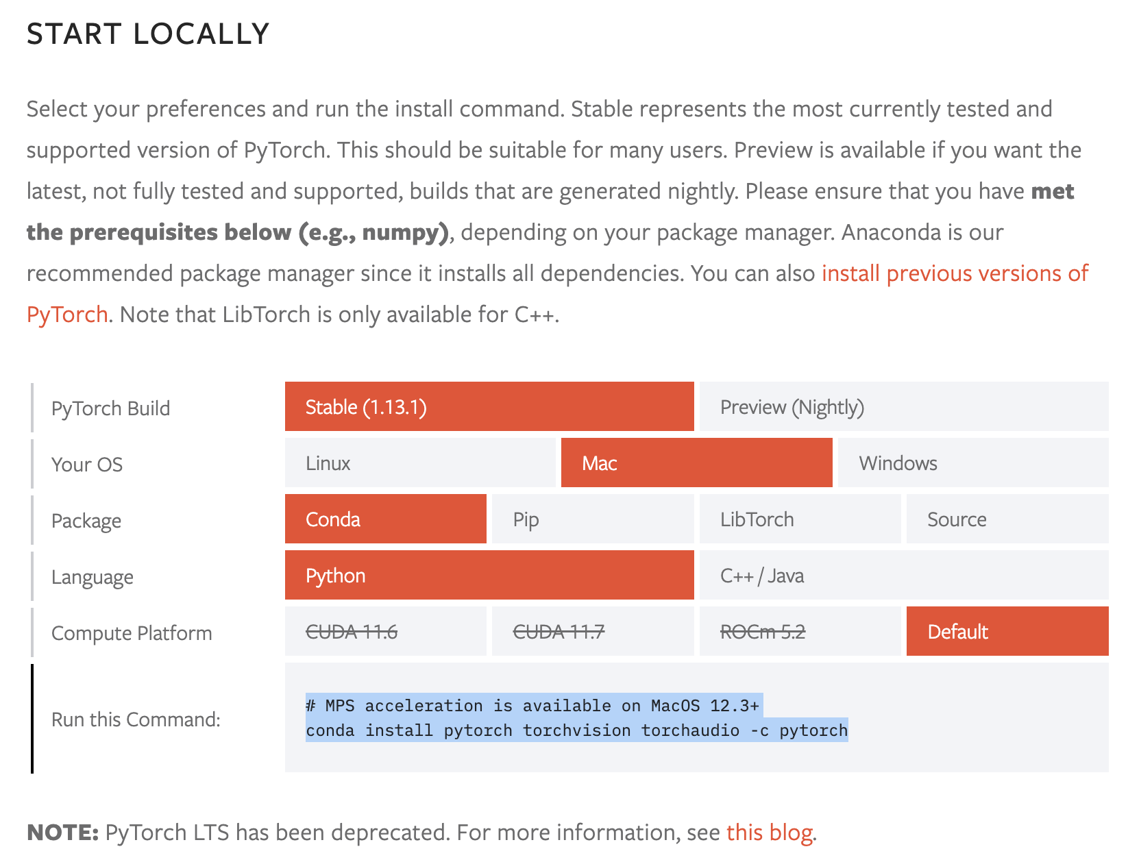
$ conda activate py310
# MPS acceleration is available on MacOS 12.3+
$ conda install pytorch torchvision torchaudio -c pytorch
Also install tensorboard:
$ pip install tensorboard
The following example is from PyTorch. I add some explanations to make it more easily to read.
Prepare Data
PyTorch has two primitives to work with data: torch.utils.data.DataLoader and torch.utils.data.Dataset. Dataset stores the samples and their corresponding labels, and DataLoader wraps an iterable around the Dataset.
import torch
from torch import nn
from torch.utils.data import DataLoader
from torchvision import datasets
from torchvision.transforms import ToTensor

# Download training data from open datasets.
training_data = datasets.FashionMNIST(
    root="data",
    train=True,
    download=True,
    transform=ToTensor(),
)

# Download test data from open datasets.
test_data = datasets.FashionMNIST(
    root="data",
    train=False,
    download=True,
    transform=ToTensor(),
)
batch_size = 64

# Create data loaders.
train_dataloader = DataLoader(training_data, batch_size=batch_size)
test_dataloader = DataLoader(test_data, batch_size=batch_size)

for X, y in test_dataloader:
	print(f"Shape of X [N, C, H, W]: {X.shape}")
	print(f"Shape of y: {y.shape} {y.dtype}")
	break
Run the above code, you should see something like:
Shape of X [N, C, H, W]: torch.Size([64, 1, 28, 28])
Shape of y: torch.Size([64]) torch.int64
Activate Acceleration
To accelerate operations in the neural network, we move it to the GPU if available.
device = "cuda" if torch.cuda.is_available() else "mps" if torch.backends.mps.is_available() else "cpu"
print(f"Using {device} device")
Run the above code, you should see something like:
Using mps device
Build A Network
Create a module that inheritates torch.nn.Module, and override the following methods:
__init__(): Define Layer、Hyperparameters here.forward(): Define the way we do Forward Propagation.
# Define model
class NeuralNetwork(nn.Module):
    def __init__(self):
        super().__init__()
        self.flatten = nn.Flatten()
        self.linear_relu_stack = nn.Sequential(
            nn.Linear(28*28, 512),
            nn.ReLU(),
            nn.Linear(512, 512),
            nn.ReLU(),
            nn.Linear(512, 10)
        )

    def forward(self, x):
        x = self.flatten(x)
        logits = self.linear_relu_stack(x)
        return logits

model = NeuralNetwork().to(device)
print(model)
Run the above code, you should see something like:
NeuralNetwork(
  (flatten): Flatten(start_dim=1, end_dim=-1)
  (linear_relu_stack): Sequential(
    (0): Linear(in_features=784, out_features=512, bias=True)
    (1): ReLU()
    (2): Linear(in_features=512, out_features=512, bias=True)
    (3): ReLU()
    (4): Linear(in_features=512, out_features=10, bias=True)
  )
)
Optimizing the Model Parameters
To train a model, we need a $\color{blue}{\textbf{loss function}}$ and an $\color{blue}{\textbf{optimizer}}$.
loss_fn = nn.CrossEntropyLoss()
optimizer = torch.optim.SGD(model.parameters(), lr=1e-3)
In a single training loop, the model makes predictions on the training dataset (fed to it in batches), and backpropagates the prediction error to adjust the model’s parameters.
def train(dataloader, model, loss_fn, optimizer):
    size = len(dataloader.dataset)
    model.train()
    for batch, (X, y) in enumerate(dataloader):
        X, y = X.to(device), y.to(device)

        # Compute prediction error
        pred = model(X)
        loss = loss_fn(pred, y)

        # Backpropagation
        optimizer.zero_grad()
        loss.backward()
        optimizer.step()

        if batch % 100 == 0:
            loss, current = loss.item(), batch * len(X)
            print(f"loss: {loss:>7f}  [{current:>5d}/{size:>5d}]")
We also check the model’s performance against the test dataset to ensure it is learning.
def test(dataloader, model, loss_fn):
    size = len(dataloader.dataset)
    num_batches = len(dataloader)
    model.eval()
    test_loss, correct = 0, 0
    with torch.no_grad():
        for X, y in dataloader:
            X, y = X.to(device), y.to(device)
            pred = model(X)
            test_loss += loss_fn(pred, y).item()
            correct += (pred.argmax(1) == y).type(torch.float).sum().item()
    test_loss /= num_batches
    correct /= size
    print(f"Test Error: \n Accuracy: {(100*correct):>0.1f}%, Avg loss: {test_loss:>8f} \n")
The training process is conducted over several iterations (epochs). During each epoch, the model learns parameters to make better predictions. We print the model’s accuracy and loss at each epoch; we’d like to see the accuracy increase and the loss decrease with every epoch.
epochs = 5
for t in range(epochs):
    print(f"Epoch {t+1}\n-------------------------------")
    train(train_dataloader, model, loss_fn, optimizer)
    test(test_dataloader, model, loss_fn)
print("Done!")
Run the above code, you should see something like:
Epoch 1
-------------------------------
loss: 2.292424  [    0/60000]
loss: 2.284307  [ 6400/60000]
loss: 2.273162  [12800/60000]
loss: 2.273963  [19200/60000]
loss: 2.247078  [25600/60000]
loss: 2.224077  [32000/60000]
loss: 2.232416  [38400/60000]
loss: 2.198098  [44800/60000]
loss: 2.190900  [51200/60000]
loss: 2.173852  [57600/60000]
Test Error:
 Accuracy: 45.4%, Avg loss: 2.160043
Epoch 1
-------------------------------
loss: 2.292424 [ 0/60000]
loss: 2.284307 [ 6400/60000]
loss: 2.273162 [12800/60000]
loss: 2.273963 [19200/60000]
loss: 2.247078 [25600/60000]
loss: 2.224077 [32000/60000]
loss: 2.232416 [38400/60000]
loss: 2.198098 [44800/60000]
loss: 2.190900 [51200/60000]
loss: 2.173852 [57600/60000]
Test Error:
Accuracy: 45.4%, Avg loss: 2.160043
Epoch 2
-------------------------------
loss: 2.159607  [    0/60000]
loss: 2.149667  [ 6400/60000]
loss: 2.100949  [12800/60000]
loss: 2.122075  [19200/60000]
loss: 2.068469  [25600/60000]
loss: 2.011612  [32000/60000]
loss: 2.051033  [38400/60000]
loss: 1.970963  [44800/60000]
loss: 1.973816  [51200/60000]
loss: 1.919670  [57600/60000]
Test Error:
 Accuracy: 53.6%, Avg loss: 1.902983
Epoch 3
-------------------------------
loss: 1.921639  [    0/60000]
loss: 1.891842  [ 6400/60000]
loss: 1.787125  [12800/60000]
loss: 1.836427  [19200/60000]
loss: 1.716476  [25600/60000]
loss: 1.671400  [32000/60000]
loss: 1.708689  [38400/60000]
loss: 1.605900  [44800/60000]
loss: 1.635701  [51200/60000]
loss: 1.539352  [57600/60000]
Test Error:
 Accuracy: 61.3%, Avg loss: 1.539101
Epoch 4
-------------------------------
loss: 1.594801  [    0/60000]
loss: 1.558597  [ 6400/60000]
loss: 1.422635  [12800/60000]
loss: 1.494758  [19200/60000]
loss: 1.363683  [25600/60000]
loss: 1.364729  [32000/60000]
loss: 1.383241  [38400/60000]
loss: 1.308365  [44800/60000]
loss: 1.346497  [51200/60000]
loss: 1.246566  [57600/60000]
Test Error:
 Accuracy: 64.3%, Avg loss: 1.262753
Epoch 5
-------------------------------
loss: 1.334898  [    0/60000]
loss: 1.314686  [ 6400/60000]
loss: 1.163017  [12800/60000]
loss: 1.261862  [19200/60000]
loss: 1.132383  [25600/60000]
loss: 1.158551  [32000/60000]
loss: 1.178075  [38400/60000]
loss: 1.117890  [44800/60000]
loss: 1.160267  [51200/60000]
loss: 1.072705  [57600/60000]
Test Error:
 Accuracy: 65.5%, Avg loss: 1.089182